Code
import pandas as pd⬅️ Previous Session | 🏠 Course Home | 🚦 EDS217 Vibes | ➡️ Next Session |

Pandas (“Python Data Analysis Library”) is arguably the most important tool for data scientists using Python. As the central component of the Python data science toolkit, pandas is essentially where your data will “live” when you’re working in Python. Pandas is built on NumPy, which means that many of the data structures of NumPy are used in pandas. Data stored in pandas DataFrames are often analysed statistically in SciPy, visualized using plotting functions from Matplotlib, and fed into machine learning algorithms in scikit-learn.
This session will cover the basics of pandas, including DataFrame construction, importing data with pandas, DataFrame attributes, working with datetime objects, and data selection and manipulation. While this tutorial is designed to give you an overview of pandas, the docs should the first place you look for more detailed information and additional pandas functionality. The pandas documentation is particularly well-written, making it easy to find methods and functions with numerous examples. Make the docs your best friend! 🐼
The Pandas library was originally developed by Wes McKinney, who is the author of the excellent Python for Data Analysis book, which is now its third edition.
Session TopicsSeries and DataFrame objects
Series and DataFrame objects from scratch
pd.read_csv()
DataFrame attributes
df.iloc
df.loc
Datetime objects
datetime objects
We will work through this notebook together. To run a cell, click on the cell and press “Shift” + “Enter” or click the “Run” button in the toolbar at the top.
🐍 This symbol designates an important note about Python structure, syntax, or another quirk.
▶️ This symbol designates a cell with code to be run.
✏️ This symbol designates a partially coded cell with an example.

As always, we must begin by importing the pandas library. The standard import statement for pandas is:
import pandas as pd▶️ <b> Run the cell below. </b>import pandas as pdSeries and DataFrame objectsThe core components of pandas are the Series and the DataFrame objects. Both of these are essentially enhanced versions of the NumPy array, with a few key differences: 1) pandas DataFrames can be heterogeneous, meaning that the columns can contain different data types; and 2) the rows and columns of DataFrames can be identified with labels (usually strings) in addition to standard integer indexing.
A Series is essentially a column of data, while a DataFrame is a multidimensional table made up of many Series, not unlike a spreadsheet:
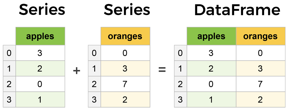
Series and DataFrames are similar in many respects – most common operations can be performed on both objects, though Series are more limited, as they can only ever contain a single column (i.e. you cannot turn a Series into a DataFrame by adding a column).
Both Series and DataFrame objects contain an Index object similar to the row index of the ndarray or the index of a list. The pandas Index object can be conceptualized as an immutable array or an ordered multiset. Unless explicitly defined otherwise, the Index of a Series or DataFrame is initialized as the ordered set of positive integers beginning at 0 (see figure above).
Series and DataFrame objects from scratchA Series can be easily created from a list or array as follows:
# Create a Series from a list
series = pd.Series([25.8, 16.2, 17.9, 18.8, 23.6, 29.9, 23.6, 22.1])

seriesseries = pd.Series([5, 6, 7, '2.4', 5, 34, 67])
series[1]
series
0    25.8
1    16.2
2    17.9
3    18.8
4    23.6
5    29.9
6    23.6
7    22.1
dtype: float64
There are many ways to create a DataFrame, but the most common are to use a list of lists or a dictionary. First, let’s use a list of lists (or an array):
# Create a df from a list of lists
df = pd.DataFrame([[25.8, 28.1, 16.2, 11.0],[17.9, 14.2, 18.8, 28.0],
                   [23.6, 18.4, 29.9, 27.8],[23.6, 36.2, 22.1, 14.5]],
columns=['A','B','C','D'])df = pd.DataFrame([[25.8, 29.4, 25.6, 54.6],
[34.5, 78.2, 86.2, 99.0],
[12.4, 75.4, 23.6, 88.5]],columns=['A', 'B', 'C', 'D'])
dfdf
      A     B     C     D
0  25.8  28.1  16.2  11.0
1  17.9  14.2  18.8  28.0
2  23.6  18.4  29.9  27.8
3  23.6  36.2  22.1  14.5
Much like with NumPy arrays, each inner list element in the outer list corresponds to a row. Using the optional columns keyword argument, we can specify the name of each column. If this parameter is not passed, the columns would be displayed with integer index values (like the rows).
Next, let’s create a DataFrame from a dict object:
# Create a df from a dictionary
df = pd.DataFrame({'A': [25.8, 17.9, 23.6, 23.6],
                   'B': [28.1, 14.2, 18.4, 36.2],
                   'C': [16.2, 18.8, 29.9, 22.1],
                   'D': [11.0, 28.0, 27.8, 14.5]})

df#df = pd.DataFrame([[25.8, 29.4, 25.6, 54.6],
# [34.5, 78.2, 86.2, 99.0],
# [12.4, 75.4, 23.6, 88.5]],columns=['A', 'B', 'C', 'D'])
df = pd.DataFrame({
'A':[25.8, 34.5, 12.4],
'B':[29.4, 78.2, 75.4],
'C':[25.6, 86.2, 23.6],
'D':[54.6, 99.0, 88.5]
})
df
      A     B     C     D
0  25.8  28.1  16.2  11.0
1  17.9  14.2  18.8  28.0
2  23.6  18.4  29.9  27.8
3  23.6  36.2  22.1  14.5
Using this method, each key corresponds to a column name, and each value is a column.
While you will likely create many DataFrames from scratch throughout your code, in most cases, you’ll have some data you’d like to import as a starting point. Pandas has several functions to read in data from a variety of formats. For now, we’ll focus on reading in data from plain-text flat files.
Most environmental datasets are stored as flat files, meaning that the data are unstructured – the records follow a uniform format, but they are not indexed and no information about relationships between records is included. Plain-text flat files use delimiters such as commas, tabs, or spaces to separate values. Pandas has a few different functions to import flat files, but perhaps the most useful is the pd.read_csv() function, designed to read CSV files. As its name suggests, a CSV (Comma Separated Values) file is a plain-text file that uses commas to delimit (separate) values. Each line of the file is a record (row).
Let’s start by taking a look at the pd.read_csv() function.
▶️ <b> Run the cell below. </b>help(pd.read_csv)As you can see, pd.read_csv() has quite a few parameters. Don’t be overwhelmed – most of these are optional arguments that allow you to specify exactly how your data file is structured and which part(s) you want to import. In particular, the sep parameter allows the user to specify the type of delimiter used in the file. The default is a comma, but you can actually pass other common delimiters (such as sep='\t', which is a tab) to import other delimited files. The only required argument is a string specifying the filepath of your file.
In this session, we’ll be importing a CSV file containing radiation data for October 2019 from a Baseline Surface Radiation Network (BSRN) station in Southern Africa. BSRN is a Global Energy and Water Cycle Experiment project aimed at monitoring changes in the Earth’s surface radiation field. The network is comprised of 64 stations across various climate zones across the globe, whose data are used as the global baseline for surface radiation by the Global Climate Observing System.
The CSV file is located in the data folder on the course GitHub repository. The files should already by in your private repo.
While the file may not display properly in VSCode, the first 10 lines of the file should look like:
DATE,H_m,SWD_Wm2,STD_SWD,DIR_Wm2,STD_DIR,DIF_Wm2,STD_DIF,LWD_Wm2,STD_LWD,SWU_Wm2,LWU_Wm2,T_degC,RH,P_hPa
2019-10-01 00:00:00,2,-3,0,0,0,-3,0,300,0.1,0,383,16.2,30.7,966
2019-10-01 00:01:00,2,-3,0,0,0,-3,0,300,0.3,0,383,16.4,30.7,966
2019-10-01 00:02:00,2,-3,0,0,0,-3,0,300,0.2,0,383,16.5,30.5,966
2019-10-01 00:03:00,2,-3,0,0,0,-3,0,300,0.1,0,383,16.5,30.4,966
2019-10-01 00:04:00,2,-3,0,0,0,-3,0,300,0.1,0,383,16.8,30.5,966
2019-10-01 00:05:00,2,-2,0,0,0,-2,0,300,0.2,0,383,16.9,30.5,966
2019-10-01 00:06:00,2,-2,0,0,0,-2,0,300,0.2,0,383,16.8,30.4,966
2019-10-01 00:07:00,2,-2,0,0,0,-2,0,300,0.1,0,384,17,31,966
2019-10-01 00:08:00,2,-2,0,0,0,-2,0,300,0.2,0,384,16.7,30.6,966
The first line of the file contains the names of the columns, which are described in the table below.
| Column name | Description |
|---|---|
| DATE | Date/Time |
| H_m | Height of measurement (\text{m}) |
| SWD_Wm2 | Incoming shortwave radiation (\text{W m}^{-2}) |
| STD_SWD | Standard deviation of incoming shortwave radiation (\text{W m}^{-2}) |
| DIR_Wm2 | Direct radiation (\text{W m}^{-2}) |
| STD_DIR | Standard deviation of direct radiation (\text{W m}^{-2}) |
| DIF_Wm2 | Diffuse radiation (\text{W m}^{-2}) |
| STD_DIF | Standard deviation of diffuse radiation (\text{W m}^{-2}) |
| LWD_Wm2 | Incoming longwave radiation (\text{W m}^{-2}) |
| STD_LWD | Standard deviation of incoming longwave radiation (\text{W m}^{-2}) |
| SWU_Wm2 | Outgoing shortwave radiation (\text{W m}^{-2}) |
| LWU_Wm2 | Outgoing longwave radiation (\text{W m}^{-2}) |
| T_degC | Air temperature (^{\circ}\text{C}) |
| RH | Relative humidity (\%) |
| P_hPa | Air pressure (\text{hPa}) |
We can import the data into pandas using the following syntax:
bsrn = pd.read_csv('../data/BSRN_GOB_2019-10.csv')✏️ <b> Try it. </b>
Copy and paste the code above to import the data in the CSV file into a pandas <code>DataFrame</code> named <code>bsrn</code>.bsrn = pd.read_csv('../data/BSRN_GOB_2019-10.csv')
bsrn
Before we move on into viewing and operating on the DataFrame, it’s worth noting that data import is rarely ever this straightforward. Most raw data require considerable cleaning before they are ready for analysis. Often some of this must happen outside of Python to format the data for import, but ideally the majority of data preprocessing can be conducted in Python – allowing you to perform the same operations on multiple datasets at once and making the process easily repeatable.
Now that we’ve loaded in our data, it would be useful to take a look at it. Given the size of our bsrn DataFrame, however, we can’t simply print out the entire table. The df.head() method allows us to quickly view the first five rows.
▶️ <b> Run the cell below. </b>bsrn.head(1)Similarly, df.tail() prints the last five rows.
▶️ <b> Run the cell below. </b>bsrn.tail()Both df.head() and df.tail() can also accept an integer argument, e.g. df.head(n), where the first n rows will be printed.
✏️ <b> Try it. </b>
Print the first and last 10 rows of <code>bsrn</code> using <code>df.head()</code> and <code>df.tail()</code>.In addition to those for viewing your data, pandas has several methods to describe attributes of your DataFrame. For example, df.info() provides basic information about the DataFrame:
▶️ <b> Run the cell below. </b>bsrn.info()The df.info() method provides several different pieces of information about the DataFrame that are sometimes useful to retrieve separately. For example, df.index returns the index as an iterable object for use in plotting and the df.columns method returns the column names as an index object which can be used in a for loop or to reset the column names. These and other descriptive DataFrame methods are summarized in the table below.
| Method | Description |
|---|---|
| df.info() | Prints a concise summary of the DataFrame |
| df.head(n) | Returns the first n rows of the DataFrame |
| df.tail(n) | Returns the last n rows of the DataFrame |
| df.index | Returns the index range (number of rows) |
| df.columns | Returns the column names |
| df.dtypes | Returns a Series with the data types of each column indexed by column name |
| df.size | Returns the total number of values in the DataFrame as an int |
| df.shape | Returns the shape of the DataFrame as a tuple (rows,columns) |
| df.values | Returns the DataFrame values as a NumPy array (not recommended) |
| df.describe() | Returns a DataFrame with summary statistics of each column |
Because DataFrames can contain labels as well as indices, indexing in pandas DataFrames is a bit more complicated than we’ve seen with strings, lists, and arrays. Generally speaking, pandas allows indexing by either the integer index or the label, but the syntax is a bit different for each.
The index operator, which refers to the square brackets following an object [], does not work quite like we might expect it to.
▶️ <b> Run the cell below. </b>bsrn.iloc[-6:,-3:]Instead of a value, we get a KeyError. This is because the Index object in pandas is essentially a dictionary, and we have not passed proper keys.
Instead, pandas uses df.iloc[] for integer-based indexing to select data by position:
bsrn.iloc[1434,12]>>> 19.6
df.iloc acts just like the index operator works with arrays. In addition to indexing a single value, df.iloc can be used to select multiple rows and columns via slicing: df.iloc[row_start:row_end:row_step, col_start:col_end:col_step].
# Select 6 rows, last 3 columns
bsrn.iloc[1434:1440,12:]
T_degC RH P_hPa 1434 19.6 17.6 965 1435 19.5 17.5 965 1436 19.4 17.4 965 1437 19.1 17.5 965 1438 19.4 17.6 965 1439 19.3 17.5 965
# First 5 columns, every 40th row
bsrn.iloc[::40,:5]
[1116 rows x 5 columns]DATE H_m SWD_Wm2 STD_SWD DIR_Wm2 0 2019-10-01 00:00:00 2 -3.0 0.0 0.0 40 2019-10-01 00:40:00 2 -3.0 0.0 0.0 80 2019-10-01 01:20:00 2 -3.0 0.0 0.0 120 2019-10-01 02:00:00 2 -3.0 0.0 0.0 160 2019-10-01 02:40:00 2 -2.0 0.0 0.0 … … … … … … 44440 2019-10-31 20:40:00 2 -2.0 0.0 0.0 44480 2019-10-31 21:20:00 2 -2.0 0.0 0.0 44520 2019-10-31 22:00:00 2 -2.0 0.0 0.0 44560 2019-10-31 22:40:00 2 -2.0 0.0 0.0 44600 2019-10-31 23:20:00 2 -2.0 0.0 0.0
In addition to df.iloc, rows of a DataFrame can be accessed using df.loc, which “locates” rows based on their labels. Unless you have set a custom index (which we will see later), the row “labels” are the same as the integer index.
When indexing a single row, df.loc (like df.iloc) transforms the row into a Series, with the column names as the index:
# Classic indexing
bsrn.loc[1434]
DATE 2019-10-01 23:54:00 H_m 2 SWD_Wm2 -2 STD_SWD 0 DIR_Wm2 0 STD_DIR 0 DIF_Wm2 -2 STD_DIF 0 LWD_Wm2 307 STD_LWD 0.1 SWU_Wm2 0 LWU_Wm2 385 T_degC 19.6 RH 17.6 P_hPa 965 Name: 1434, dtype: object
one_row = bsrn.loc[0]
one_row🐍 <b>DataFrames + data types.</b> Notice that the <code>dtype</code> of the Series is an <code>object</code>. This is because the column contains mixed data types – floats, integers, and an <code>object</code> in the first row. Unlike NumPy, pandas allows both rows and columns to contain mixed data types. However, while it is perfectly fine (and, in fact, almost always necessary) to have multiple data types within a single <b><i>row</i></b>, it is best if each <b><i>column</i></b> is comprised of a <b><i>single data type</i></b>.Slicing using df.loc is similar to df.iloc, with the exception that the stop value is inclusive:
# Using .loc
bsrn.loc[1434:1440]
[7 rows x 15 columns]DATE H_m SWD_Wm2 STD_SWD DIR_Wm2 … SWU_Wm2 LWU_Wm2 T_degC RH P_hPa 1434 2019-10-01 23:54:00 2 -2.0 0.0 0.0 … 0 385 19.6 17.6 965 1435 2019-10-01 23:55:00 2 -2.0 0.0 0.0 … 0 385 19.5 17.5 965 1436 2019-10-01 23:56:00 2 -2.0 0.0 0.0 … 0 386 19.4 17.4 965 1437 2019-10-01 23:57:00 2 -2.0 0.0 0.0 … 0 386 19.1 17.5 965 1438 2019-10-01 23:58:00 2 -2.0 0.0 0.0 … 0 386 19.4 17.6 965 1439 2019-10-01 23:59:00 2 -2.0 0.0 0.0 … 0 386 19.3 17.5 965 1440 2019-10-02 00:00:00 2 -2.0 0.0 0.0 … 0 386 19.1 17.5 965
In addition to integer indexing with df.iloc, columns can be accessed in two ways: dot notation . or square brackets []. The former takes advantage of the fact that the columns are effectively “attributes” of the DataFrame and returns a Series:
bsrn.SWD_Wm2
0 -3.0 1 -3.0 2 -3.0 3 -3.0 4 -3.0 ... 44635 -2.0 44636 -2.0 44637 -2.0 44638 -2.0 44639 -2.0 Name: SWD_Wm2, Length: 44640, dtype: float64
The second way of extracting columns is to pass the column name as a string in square brackets, i.e. df['col']:
bsrn['SWD_Wm2']
0 -3.0 1 -3.0 2 -3.0 3 -3.0 4 -3.0 ... 44635 -2.0 44636 -2.0 44637 -2.0 44638 -2.0 44639 -2.0 Name: SWD_Wm2, Length: 44640, dtype: float64
Using single brackets, the result is a Series. However, using double brackets, it is possible to return the column as a DataFrame:
bsrn[['SWD_Wm2']]
[44640 rows x 1 columns]SWD_Wm2 0 -3.0 1 -3.0 2 -3.0 3 -3.0 4 -3.0 … … 44635 -2.0 44636 -2.0 44637 -2.0 44638 -2.0 44639 -2.0
This allows you to add additional columns, which you cannot do with a Series object. Furthermore, with the double bracket notation, a list is being passed to the index operator (outer brackets). Thus, it is possible to extract multiple columns by adding column names to the list:
new_df = bsrn[['H_m', 'T_degC']]
new_df.head()bsrn[['SWD_Wm2','LWD_Wm2']]
[44640 rows x 2 columns]SWD_Wm2 LWD_Wm2 0 -3.0 300.0 1 -3.0 300.0 2 -3.0 300.0 3 -3.0 300.0 4 -3.0 300.0 … … … 44635 -2.0 380.0 44636 -2.0 380.0 44637 -2.0 380.0 44638 -2.0 381.0 44639 -2.0 381.0
When accessing a single column, the choice between using dot notation and square brackets is more or less a matter of preference. However, there are occasions when the bracket notation proves particularly useful. For example, you could access each column in a DataFrame by iterating through df.columns, which returns an Index object containing the column names as str objects that can be directly passed to the index operator. Additionally, you may find it useful to use the double bracket syntax to return a DataFrame object, rather than a Series, which can only ever contain a single column of data.
bsrn.info()Datetime objectsLike the BSRN data we are working with in this session, many environmental datasets include timed records. Python has a few different libraries for dealing with timestamps, which are referred to as datetime objects. The standard datetime library is the primary way of manipulating dates and times in Python, but there are additional third-party packages that provide additional support. A few worth exploring are dateutil, an extension of the datetime library useful for parsing timestamps, and pytz, which provides a smooth way of tackling time zones.
Though we will not review datetime objects in depth here, it is useful to understand the basics of how to deal with datetime objects in Python as you will no doubt encounter them in the future. For now, we will focus on a few pandas functions built on the datetime library to handle datetime objects.
The pd.date_range() function allows you to build a DatetimeIndex with a fixed frequency. This can be done by specifying a start date and an end date as follows:
pd.date_range('4/1/2017','4/30/2017')
>>> DatetimeIndex(['2017-01-01', '2017-01-02', '2017-01-03', '2017-01-04',
'2017-01-05', '2017-01-06', '2017-01-07', '2017-01-08',
'2017-01-09', '2017-01-10',
...
'2020-12-22', '2020-12-23', '2020-12-24', '2020-12-25',
'2020-12-26', '2020-12-27', '2020-12-28', '2020-12-29',
'2020-12-30', '2020-12-31'],
dtype='datetime64[ns]', length=1461, freq='D')Because it was not specified otherwise, the frequency was set as the default, daily. To return a different frequency, we could use the freq parameter:
# Specify start and end, minute-ly frequency
pd.date_range('1/1/2017','12/31/2020', freq='min')
>>> DatetimeIndex(['2017-01-01 00:00:00', '2017-01-01 00:01:00',
'2017-01-01 00:02:00', '2017-01-01 00:03:00',
'2017-01-01 00:04:00', '2017-01-01 00:05:00',
'2017-01-01 00:06:00', '2017-01-01 00:07:00',
'2017-01-01 00:08:00', '2017-01-01 00:09:00',
...
'2020-12-30 23:51:00', '2020-12-30 23:52:00',
'2020-12-30 23:53:00', '2020-12-30 23:54:00',
'2020-12-30 23:55:00', '2020-12-30 23:56:00',
'2020-12-30 23:57:00', '2020-12-30 23:58:00',
'2020-12-30 23:59:00', '2020-12-31 00:00:00'],
dtype='datetime64[ns]', length=2102401, freq='T')
# Specify start and end, monthly frequency
pd.date_range('1/1/2017','12/31/2020', freq='M')
>>> DatetimeIndex(['2017-01-31', '2017-02-28', '2017-03-31', '2017-04-30',
'2017-05-31', '2017-06-30', '2017-07-31', '2017-08-31',
'2017-09-30', '2017-10-31', '2017-11-30', '2017-12-31',
'2018-01-31', '2018-02-28', '2018-03-31', '2018-04-30',
'2018-05-31', '2018-06-30', '2018-07-31', '2018-08-31',
'2018-09-30', '2018-10-31', '2018-11-30', '2018-12-31',
'2019-01-31', '2019-02-28', '2019-03-31', '2019-04-30',
'2019-05-31', '2019-06-30', '2019-07-31', '2019-08-31',
'2019-09-30', '2019-10-31', '2019-11-30', '2019-12-31',
'2020-01-31', '2020-02-29', '2020-03-31', '2020-04-30',
'2020-05-31', '2020-06-30', '2020-07-31', '2020-08-31',
'2020-09-30', '2020-10-31', '2020-11-30', '2020-12-31'],
dtype='datetime64[ns]', freq='M')There are many other parameters for the pd.date_range() function, as well as other pandas functions. More useful to us, however, are the functions for dealing with existing timestamps, such as those in our bsrn DataFrame.
Let’s start by taking a look at bsrn.DATE, which contains the timestamps for each record of our BSRN data.
bsrn.DATE
0 2019-10-01 00:00:00 1 2019-10-01 00:01:00 2 2019-10-01 00:02:00 3 2019-10-01 00:03:00 4 2019-10-01 00:04:00 ... 44635 2019-10-31 23:55:00 44636 2019-10-31 23:56:00 44637 2019-10-31 23:57:00 44638 2019-10-31 23:58:00 44639 2019-10-31 23:59:00 Name: DATE, Length: 44640, dtype: object
While the values certainly resemble datetime objects, they are stored in pandas as “objects,” which basically means that pandas doesn’t recognize the data type – it doesn’t know how to handle them. Using the pd.to_datetime() function, we can convert this column to datetime objects:
pd.to_datetime(bsrn.DATE)
0 2019-10-01 00:00:00 1 2019-10-01 00:01:00 2 2019-10-01 00:02:00 3 2019-10-01 00:03:00 4 2019-10-01 00:04:00 ... 44635 2019-10-31 23:55:00 44636 2019-10-31 23:56:00 44637 2019-10-31 23:57:00 44638 2019-10-31 23:58:00 44639 2019-10-31 23:59:00 Name: DATE, Length: 44640, dtype: datetime64[ns]
Notice that ostensibly nothing has changed, but the dtype is now a datetime object, making it much easier to manipulate not only this column, but the entire DataFrame. For instance, now that we’ve told pandas that this column contains timestamps, we can set this column as the index using df.set_index().
▶️ <b> Run the cell below. </b># Convert bsrn.DATE column to datetime objects
bsrn = pd.read_csv('../data/BSRN_GOB_2019-10.csv')

bsrn['DATE'] = pd.to_datetime(bsrn.DATE) # Note: overwriting a column like this is NOT recommended.
# Set bsrn.DATE as the DataFrame index
bsrn.set_index('DATE', inplace=True)
bsrn.head()As noted in the comment in the cell above, reseting the values in a column as we did in the first line of code is generally not recommended, but in this case, since we knew exactly what the result would be, it’s acceptable. Also, notice the inplace=True argument passed to df.set_index(). This prevented us from having to copy the DataFrame to a new variable, instead performing the operation in-place.
Let’s take a look at our DataFrame again:
▶️ <b> Run the cell below. </b>bsrn.info()As expected, the index has been changed to a DatetimeIndex, and there is no longer a 'DATE' column. Had we wanted to keep the timestamps as a column as well, we could have passed drop=False to df.set_index(), telling pandas not to drop (or delete) the 'DATE' column. We can look at the DatetimeIndex just as before using df.index.
▶️ <b> Run the cell below. </b>bsrn.describe()Now that we have a DatetimeIndex, we can access specific attributes of the datetime objects like the year, day, hour, etc. To do this, we add the desired time period using dot notation: df.index.attribute. For a full list of attributes, see the pd.DatetimeIndex documentation. For example:
# Get the hour of each record
bsrn.index.hour
Int64Index([ 0,  0,  0,  0,  0,  0,  0,  0,  0,  0,
...
23, 23, 23, 23, 23, 23, 23, 23, 23, 23],
dtype='int64', name='DATE', length=44640)
bsrn.index.unique()The result is a pandas Index object with the same length as the original DataFrame. To return only the unique values, we use the Series.unique() function, which can be used on any Series object (including a column of a DataFrame):
# Get the unique hour values
bsrn.index.hour.unique()
Int64Index([ 0,  1,  2,  3,  4,  5,  6,  7,  8,  9, 10, 11, 12, 13, 14, 15, 16,
17, 18, 19, 20, 21, 22, 23],
dtype='int64', name='DATE')
🐍 <b>Method chaining.</b> This process of stringing multiple methods together in a single line of code is called <b>method chaining</b>, a hallmark of object-oriented programming. Method chaining is a means of concatenating functions in order to quickly complete a series of data transformations. In pandas, we often use method chaining in aggregation processes to perfrom calculations on groups or selections of data. Methods are appended using dot notation to the end of a command. Any code that is expressed using method chaining could also be written using a series of commands (and vice versa). Method chaining is common in JavaScript, and while it is not widely used in Python, it is commonly applied in pandas.Dealing with datetime objects can be tricky and often requires a bit of trial and error before the timestamps are in the desired format. If you know the format of your dataset and its timestamp records, you can parse the datetimes and set the index when reading in the data. For example, we could have imported our data as follows:
bsrn = pd.read_csv('../data/BSRN_GOB_2019-10.csv',index_col=0,parse_dates=True)This would have accomplished what we ultimately did in three lines in a single line of code. But remember, working with most raw datasets is rarely this straightforward – even the file we are using in this session was preprocessed to streamline the import process!
bsrn = pd.read_csv('../data/BSRN_GOB_2019-10.csv',index_col=0,parse_dates=True)
bsrn[['LWD_Wm2', 'SWD_Wm2']].mean()
LWD_Wm2 342.350692
SWD_Wm2 318.046516
dtype: float64Now that our DataFrame is a bit cleaner – each of the columns contains a single, numeric data type – we are ready to start working with our data. Next, we’ll explore DataFrame reduction operations, how to add and delete data, and concatenation in pandas.
DataFrame reductionMuch like NumPy, pandas has several useful methods for reducing data to a single statistic. These are intuitively named and include: df.mean(), df.median(), df.sum(), df.max(), df.min(), and df.std(). Unlike array reduction, however, these basic statistical methods in pandas operate column-wise, returning a Series containing the statistic for each column indexed by column name. For example:
# Calculate median of each column
bsrn.median()
H_m          2.0
SWD_Wm2     27.0
STD_SWD      0.3
DIR_Wm2      0.0
STD_DIR      0.0
DIF_Wm2     19.0
STD_DIF      0.1
LWD_Wm2    340.0
STD_LWD      0.1
SWU_Wm2     11.0
LWU_Wm2    432.0
T_degC      22.4
RH          33.1
P_hPa      965.0
dtype: float64
To retrieve the value for just a single column, you can use indexing to call the column as a Series:
# Calculate median incoming shortwave radiation
bsrn.SWD_Wm2.median()
>>> 27.0
Furthermore, while it is not apparent in this example, pandas default behaviour is to ignore NaN values when performing computations. This can be changed by passing skipna=False to the reduction method (e.g. df.median(skipna=False)), though skipping NaNs is often quite useful!
bsrn = pd.read_csv('../data/BSRN_GOB_2019-10.csv',index_col=0,parse_dates=True)Much like when we converted bsrn.DATE to datetime objects, a column can be added to a DataFrame using square bracket notation with a new column label as a string. The data for the new column can come in the form of a list, Series, or a single value:
df = pd.DataFrame([[25.8, 28.1, 16.2, 11.0],
                   [17.9, 14.2, 18.8, 28.0],
                   [23.6, 18.4, 29.9, 27.8],
                   [23.6, 36.2, 22.1, 14.5]],
columns=['A','B','C','D'])df = pd.DataFrame([[25.8, 28.1, 16.2, 11.0],
[17.9, 14.2, 18.8, 28.0],
[23.6, 18.4, 29.9, 27.8],
[23.6, 36.2, 22.1, 14.5]],
columns=['A','B','C','D'])df['E'] = [13.0, 40.1, 39.8, 28.2]df['F'] = pd.Series([18, 22, 30, 24])
df['G'] = 'blue'

dfdf['E'] = [34, 45, 34, 56]
df['G'] = ['blue', 'sky and a c', 'cat', 'blue']
df['F'] = df['E'] - df['E'].mean()
def has_c(s):
return s.find('c') != -1
df[df['G'].apply(has_c)]| A | B | C | D | E | G | F | A_degF | is_hot | H | |
|---|---|---|---|---|---|---|---|---|---|---|
| 1 | 17.9 | 14.2 | 18.8 | 28.0 | 45 | sky and a c | 2.75 | 64.22 | False | 28.0 |
| 2 | 23.6 | 18.4 | 29.9 | 27.8 | 34 | cat | -8.25 | 74.48 | True | 27.8 |
      A     B     C     D     E   F     G
0  25.8  28.1  16.2  11.0  13.0  18  blue
1  17.9  14.2  18.8  28.0  40.1  22  blue
2  23.6  18.4  29.9  27.8  39.8  30  blue
3  23.6  36.2  22.1  14.5  28.2  24  blue
New columns can also be added as the result of an arithmetic operation (e.g. sum, product, etc.) performed on one or more existing columns:
# Add a new column by converting values in df.A from °C to °F
df['A_degF'] = (df['A'] * (9/5)) + 32

# Add a new column representing the difference between df.B and df.C
df['BC_diff'] = df.B - df.C

df
      A     B     C     D     E   F     G  A_degF  BC_diff
0  25.8  28.1  16.2  11.0  13.0  18  blue   78.44     11.9
1  17.9  14.2  18.8  28.0  40.1  22  blue   64.22     -4.6
2  23.6  18.4  29.9  27.8  39.8  30  blue   74.48    -11.5
3  23.6  36.2  22.1  14.5  28.2  24  blue   74.48     14.1
import numpy as np

df1 = df[ # Take a dAtaframe.
    df['A'] < df['D'] # find the rows where this is true.
][['C','B']]

print(df1)
df1.mean()
C B
1 18.8 14.2
2 29.9 18.4C 24.35
B 16.30
dtype: float64Finally, you can use a Boolean expression to add a column, which contains Boolean objects (True or False) based on the condition. For example:
# Add a column with Booleans for values in df.D greater than or equal to 20.0
df['D_20plus'] = df.D >= 20.0

df
      A     B     C     D     E   F     G  A_degF  BC_diff  D_20plus
0  25.8  28.1  16.2  11.0  13.0  18  blue   78.44     11.9     False
1  17.9  14.2  18.8  28.0  40.1  22  blue   64.22     -4.6      True
2  23.6  18.4  29.9  27.8  39.8  30  blue   74.48    -11.5      True
3  23.6  36.2  22.1  14.5  28.2  24  blue   74.48     14.1     False
df['H'] = df.D[df.D >= 20]

def add_one(d):
    return d+1

df['G']
0 2
1 2
2 2
3 2
Name: G, dtype: int64These conditional expressions can also be used to create Boolean masks, which allow you to “mask” the values in the DataFrame that do not meet a condition, only extracting those that do. For example, let’s use a Boolean mask to apply an mathematical expression on only certain values in column 'D':
# Subtract 20 from all values in dfD greater than or equal to 20
df['D_less20'] = df.D[df.D >= 20.0] - 20.0

df
      A     B     C     D     E   F     G  A_degF  BC_diff  D_20plus  D_less20
0  25.8  28.1  16.2  11.0  13.0  18  blue   78.44     11.9     False       NaN
1  17.9  14.2  18.8  28.0  40.1  22  blue   64.22     -4.6      True       8.0
2  23.6  18.4  29.9  27.8  39.8  30  blue   74.48    -11.5      True       7.8
3  23.6  36.2  22.1  14.5  28.2  24  blue   74.48     14.1     False       NaN
All values that do not meet the condition are hidden from the expression, leaving NaNs in the resulting column. Boolean masks come in quite handy in data analysis, as they allow you to extract certain rows from a DataFrame based on their values in one or more columns.
Furthermore, in addition to simply adding columns, new columns can be inserted in a desired index position using df.insert() with arguments specifying the location, name, and values of the column:
# Create list of seasons
seasons = ['winter', 'spring', 'summer', 'fall']

# Insert season as first column
df.insert(0, 'SEASON', seasons)

df
   SEASON     A     B     C     D     E   F     G  A_degF  BC_diff  D_20plus  D_less20
0  winter  25.8  28.1  16.2  11.0  13.0  18  blue   78.44     11.9     False       NaN
1  spring  17.9  14.2  18.8  28.0  40.1  22  blue   64.22     -4.6      True       8.0
2  summer  23.6  18.4  29.9  27.8  39.8  30  blue   74.48    -11.5      True       7.8
3    fall  23.6  36.2  22.1  14.5  28.2  24  blue   74.48     14.1     False       NaN
Unlike adding new data columns, removing columns from a DataFrame should be done with caution. In fact, it’s not a bad idea to create a copy of your DataFrame before performing any operations. This will allow you to return to the original data as needed without having to re-import or re-initialize the DataFrame. If you do need to remove a column, you can use the del command:
# Delete 'G' from df
del df['G']

df
   SEASON     A     B     C     D     E   F  A_degF  BC_diff  D_20plus  D_less20
0  winter  25.8  28.1  16.2  11.0  13.0  18   78.44     11.9     False       NaN
1  spring  17.9  14.2  18.8  28.0  40.1  22   64.22     -4.6      True       8.0
2  summer  23.6  18.4  29.9  27.8  39.8  30   74.48    -11.5      True       7.8
3    fall  23.6  36.2  22.1  14.5  28.2  24   74.48     14.1     False       NaN
Note that this is an in-place operation, meaning that the column is deleted from the original variable. Alternatively, you can use df.pop() to extract a column. This method allows a column values to be extracted (and deleted) from a DataFrame and assigned to a new variable:
# Extract column 'F' from df as a new Series
df_F = df.pop('F')

df
   SEASON     A     B     C     D     E  A_degF  BC_diff  D_20plus  D_less20
0  winter  25.8  28.1  16.2  11.0  13.0   78.44     11.9     False       NaN
1  spring  17.9  14.2  18.8  28.0  40.1   64.22     -4.6      True       8.0
2  summer  23.6  18.4  29.9  27.8  39.8   74.48    -11.5      True       7.8
3    fall  23.6  36.2  22.1  14.5  28.2   74.48     14.1     False       NaN
In addition to manipulating individual columns, you can apply a function to an entire Series or DataFrame using the pandas function df.apply(). For example, consider our original DataFrame df, which consists of temperature values in °C:
df = pd.DataFrame([[25.8, 28.1, 16.2, 11.0],[17.9, 14.2, 18.8, 28.0],
                   [23.6, 18.4, 29.9, 27.8],[23.6, 36.2, 22.1, 14.5]],
                 columns=['A','B','C','D'])
df
      A     B     C     D
0  25.8  28.1  16.2  11.0
1  17.9  14.2  18.8  28.0
2  23.6  18.4  29.9  27.8
3  23.6  36.2  22.1  14.5
We previously used arithmetic operators to convert column 'A' to °F, but we could also use a function. First, let’s define a function convert_CtoF to convert temperature values from Celsius to Fahrenheit:
def convert_CtoF(degC):
    """ Converts a temperature to from Celsius to Fahrenheit

    Parameters
    ----------
        degC : float
            Temperature value in °C

    Returns
    -------
        degF : float
            Temperature value in °F
    """

    degF = (degC *(9./5)) + 32

    return degF
Using df.apply() we can use this function to convert values in column 'A' as follows:
df.A.apply(convert_CtoF)
0    78.44
1    64.22
2    74.48
3    74.48
Name: A, dtype: float64
Where this becomes especially useful is for operating on entire DataFrames. You have to be careful with this if your DataFrame contains multiple data types, but it works well when you need to perform an operation on an entire DataFrame. For example, we could convert all of the values in df by iterating through the columns, or, using df.apply(), we could acheive the same result in a single line of code:
df.apply(convert_CtoF)
       A      B      C      D
0  78.44  82.58  61.16  51.80
1  64.22  57.56  65.84  82.40
2  74.48  65.12  85.82  82.04
3  74.48  97.16  71.78  58.10
df.apply(convert_CtoF)
       A      B      C      D
0  78.44  82.58  61.16  51.80
1  64.22  57.56  65.84  82.40
2  74.48  65.12  85.82  82.04
3  74.48  97.16  71.78  58.10
There are several ways to combine data from multiple Series or DataFrames into a single object in pandas. These functions include pd.append(), pd.join(), and pd.merge(). We will focus on the general pd.concat() function, which is the most versatile way to concatenate pandas objects. To learn more about these other functions, refer to the pandas documentation or see Chapter 3 of the Python Data Science Handbook.
Let’s start by considering the simplest case of two DataFrames with identical columns:
df1 = pd.DataFrame([['Los Angeles', 34.0522, -118.2437],
                    ['Bamako', 12.6392, 8.0029],
                    ['Johannesburg', -26.2041, 28.0473],
                    ['Cairo', 30.0444, 31.2357]],
                  columns=['CITY', 'LAT', 'LONG'])

df2 = pd.DataFrame([['Cape Town', -33.9249, 18.4241],
                    ['Kyoto', 35.0116, 135.7681],
                    ['London', 51.5074, -0.1278],
                    ['Cochabamba', -17.4140, -66.1653]],
                  columns=['CITY', 'LAT', 'LONG'])
Using pd.concat([df1,df2]), we can combine the two DataFrames into one. Notice that we must pass the DataFrames as a list, because pd.concat() requires an iterable object as its input.
# Concatenate df1 and df2
city_coords = pd.concat([df1,df2])

city_coords
           CITY      LAT      LONG
0   Los Angeles  34.0522 -118.2437
1        Bamako  12.6392    8.0029
2  Johannesburg -26.2041   28.0473
3         Cairo  30.0444   31.2357
0     Cape Town -33.9249   18.4241
1         Kyoto  35.0116  135.7681
2        London  51.5074   -0.1278
3    Cochabamba -17.4140  -66.1653
By default, pandas concatenates along the row axis, appending the values in df2 to df1 as new rows. However, notice that the original index values have been retained. Since these index labels do not contain useful information, it would be best to reset the index before proceeding. This can be done in one of two ways. First, we could have passed ignore_index=True to the pd.concat() function, telling pandas to ignore the index labels. Since we have already created a new variable, however, let’s use a more general method: df.reset_index().
# Reset index in-place and delete old index
city_coords.reset_index(inplace=True, drop=True)

city_coords
           CITY      LAT      LONG
0   Los Angeles  34.0522 -118.2437
1        Bamako  12.6392    8.0029
2  Johannesburg -26.2041   28.0473
3         Cairo  30.0444   31.2357
4     Cape Town -33.9249   18.4241
5         Kyoto  35.0116  135.7681
6        London  51.5074   -0.1278
7    Cochabamba -17.4140  -66.1653
By passing the optional inplace and drop parameters, we ensured that pandas would reset the index in-place (the default is to return a new DataFrame) and drop the old index (the default behaviour is to add the former index as a column).
Now let’s consider the case of concatenating two DataFrames whose columns do not match. In this case, pandas will keep source rows and columns separate in the concatenated DataFrame, filling empty cells with NaN values:
df3 = pd.DataFrame([['USA', 87],['Mali', 350],['South Africa', 1753],['Egypt', 23],
                    ['South Africa', 25],['Japan', 47],['UK', 11],['Bolivia', 2558]],
                  columns=['COUNTRY', 'ELEV'])

# Concatenate cities1 and df3
pd.concat([city_coords,df3])
           CITY      LAT      LONG       COUNTRY    ELEV
0   Los Angeles  34.0522 -118.2437           NaN     NaN
1        Bamako  12.6392    8.0029           NaN     NaN
2  Johannesburg -26.2041   28.0473           NaN     NaN
3         Cairo  30.0444   31.2357           NaN     NaN
4     Cape Town -33.9249   18.4241           NaN     NaN
5         Kyoto  35.0116  135.7681           NaN     NaN
6        London  51.5074   -0.1278           NaN     NaN
7    Cochabamba -17.4140  -66.1653           NaN     NaN
0           NaN      NaN       NaN           USA    87.0
1           NaN      NaN       NaN          Mali   350.0
2           NaN      NaN       NaN  South Africa  1753.0
3           NaN      NaN       NaN         Egypt    23.0
4           NaN      NaN       NaN  South Africa    25.0
5           NaN      NaN       NaN         Japan    47.0
6           NaN      NaN       NaN            UK    11.0
7           NaN      NaN       NaN       Bolivia  2558.0
Instead, we must pass axis=1 to the function to specify that we want to add the data in df3 as columns to the new DataFrame:
# Concatenate along column axis
cities = pd.concat([city_coords,df3], axis=1)

cities
           CITY      LAT      LONG       COUNTRY  ELEV
0   Los Angeles  34.0522 -118.2437           USA    87
1        Bamako  12.6392    8.0029          Mali   350
2  Johannesburg -26.2041   28.0473  South Africa  1753
3         Cairo  30.0444   31.2357         Egypt    23
4     Cape Town -33.9249   18.4241  South Africa    25
5         Kyoto  35.0116  135.7681         Japan    47
6        London  51.5074   -0.1278            UK    11
7    Cochabamba -17.4140  -66.1653       Bolivia  2558
While you will most likely use pandas DataFrames to manipulate data, perform statistical analyses, and visualize results within Python, you may encounter scenarios where it is useful to “save” a DataFrame with which you’ve been working. Exporting data from pandas is analogous to importing it.
Let’s take the example of the cities DataFrame we created in the last example. Now that we’ve compiled GPS coordinates of various cities, let’s say we wanted to load these data into a GIS software application. We could export this DataFrame using df.to_csv() specifying the file name with the full file path as follows:
cities.to_csv('./exports/cities.csv')You made it to the end of your first journey with Pandas. You deserve a warm, fuzzy reward…
from IPython.display import YouTubeVideo
from random import choice
ids=['sGF6bOi1NfA','Z98ZxYFsIWo', 'l73rmrLTHQc', 'D7xWXk5T3-g']
YouTubeVideo(id=choice(ids),width=600,height=300)